Standing waves of UHF radio are used to measure the speed of radio waves, which we then compare with the measured speed of light. This is an important comparison: Maxwell realised that the waves that are a solution to the equations for electricity and magnetism had a speed similar to that measured for light. This was persuasive evidence that light was an electromagnetic wave. This page supports the multimedia tutorial The Nature of Light.
For
this experiment, we set up a horizontal dipole antenna on a pole and powered it with a 300 MHz
oscillator to radiate UHF radio waves. A second
dipole antenna in my hand is connected to the oscilloscope whose screen we see at left.
The wavelength is one metre, so both antenna are one half a wavelength long.
The waves are transverse and are polarised with the electric field parallel to the antenna, as we show in Transverse Electromagnetic Waves.
The antenna at the top of the pole radiates UHF. The animation shows incident (blue), reflected (red) and superposition (purple).
On the ground we have spread aluminium foil. Aluminium is a conductor, so this reflects the electric wave with a phase change of 180°, giving approximately zero electric field in the conductor. The receiving antenna measures the superposition of the incident and reflected waves. In the animation, the incident (electrical) wave is blue, the reflected wave is red, and the purple wave is the superposition: the total electric field at that point. The horizontal scale is arbitrary, the vertical scale is pretty accurate and time has been slowed down by a hundred million or so for us to see it.
The amplitude of the wave decreases as 1/r, where r is the distance from the transmitter. At the point of reflection, the incident and reflected waves have the same amplitude, but elsewhere the incident wave has a larger amplitude than the reflected one. Thus the nodes in the combined wave do not have an amplitude of zero (except at the point of reflection); rather, they are local minima in the interference pattern.
The standing wave experiment. The oscilloscope at right shows voltage produced across the receiving antenna in my hand. The purple curve is just an animation showing the superposition – see the previous section.) A metre rule is attached to the antenna pole for scale.
So here is the experiment. Two video cameras were used. They were synchronised to within a frame or two by zooming out and waving an arm in front of both. One gives the view at left, the other was focussed on the oscilloscope screen, whose (simultaneous) image was shown at right. The nodes are easiest to see near the bottom, where the incident and reflected amplitudes are most similar in amplitude.
As we saw in interference, the nodes are separated by half a wavelength, which is here L = λ/2 = 0.50 m. The oscilloscope setting had 2 ns per division, giving 20 ns across the screen. The period of the wave is measured at T = 3.3 ns (the oscillator was set at 300 MHz), so the speed is λ/T = 3.0 X 10⁸ m.s−1. (Thanks to Barry Perczuk, Pat McMillan and the UNSW third year physics lab for lending both the UHF oscillator and the 500 MHz oscilloscope.)
It's interesting to compare this measured speed of radio waves with the measured speed of light. Maxwell noted that the speed of the wave solution to the equations of electromagnetism was similar to that measured for light. This was persuasive evidence that light was an electromagnetic wave.
Light, electromagnetism, time and space
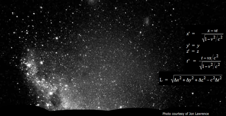
The night sky reveals light from very distant stars. Several other galaxies are, under good conditions, visible with the naked eye, and very many more are visible with telescopes that record light that has been travelling for over ten billion years. On the right are the Lorentz transformation equations and the separation of two events in space-time.
It also appears in the theory of relativity, where it is the natural conversion between time and space. In space-time, the separation betwen two events (with separations of space Δx, Δy, Δz and in time Δt) is given by
L = √(Δx2 + Δy2 + Δz2 − c2Δt2).
Electromagnetic radiation travels through space without a medium. So, in retrospect, we can say that it is perhaps unsurprising that c is the natural relation between space and time. When Lamour, Lorentz, Fitzgerald and Einstein proposed this, however, this relation was much less obvious. We give an introduction to relativity in Einsteinlight.
Electromagnetic waves
The animation below shows the electric field E and magnetic field field B of a wave propagating in one dimension.
An animation showing the electric field E and magnetic field B of a wave propagating in one dimension.
The following link takes you to page where we measure the speed of light using laser light and time-of-flight. In the next, we use the same radio apparatus to investigate the polarisation of radio waves (and of light). The next one takes you back to the multimedia tutorial The Nature of Light..