Travelling waves, superposition, reflection and transmission
Waves in a string are discussed in this support page to the multimedia chapter Travelling Waves in the volume Waves and Sound. It gives background information and further details on equations, linear media, superposition and reflection at boundaries between media with different properties.
The stretched string is mentioned in standard texts, and we shall meet it in later chapters. The film clip below shows a rope, not a string, and it is not stretched very much. As we'll see later, a relatively large mass per unit length (a rope instead of a string) and a low tension both make the wave travel more slowly, which is useful if you want to see the motion of pulses with the naked eye or a video camera, as we do here.
Why study something so impractical as a bump in a rope? Waves in strings are important in musical instruments and in engineering examples, such as supporting cables of bridges. That is not our reason, however. Rather, physicists like to start with a simple system, which we can understand easily, and then to extend our understanding to more complicated systems. Our purpose here is to understand qualitatively the physics behind the transmission of a wave pulse. This wave travels in one dimension (to the right), rather than spreading out in two or three dimensions, and it is easy to see.
So, simply by shaking the rope, I send a pulse along the rope. You'll see that the displacement is approximately in a direction perpendicular to the rope, which makes it (largely) a transverse wave. In the clip below, the arrows show the tension acting on sections of the rope on the leading edge of the pulse. I say sections, plural, because of course it is always a different section of the rope: although the pulse travels to the right, the rope 'stays where it is'. This is a very common feature of waves: a pattern of displacement travels through a medium.
So, in each frame of the clip above, the section of the rope that is, at that moment, at the very front of the pulse, is acted on by a tension applied at either end. The force at right is horizontal, that at left has a positive y component, so from Newton's second law, this segment is accelerated in the y direction. Let's now look at segments a little further back on the pulse.
On these segments, the two forces are equal and opposite. Consider one frame of the movie. In the preceding frame, the segment identified was accelerated in the positive direction. Now the force on it in the y direction is zero. So it continues travelling in the y direction.
On the segments identified here, the two forces both have negative y components. In the preceding frame, the segment identified was travelling in the y direction. Now the force on it in the y direction is in the negative direction. So it will come to rest and then reverse direction.
And finally these segments are subject to a nett force in the positive direction, which brings them to rest after the pulse has gone by. The pulse has passed by, leaving the rope in its original position. This is a general feature of waves: the pattern may move with respect to the medium.
Equations for a travelling wave
Let's now describe a travelling wave mathematically. Instead of the somewhat asymmetrical pulse produced by my moving hand, we'll consider a more idealised pulse, such as the one shown in the next animation. Here is a pulse in which a displacement in the y direction moves to the right (positive x direction) as time t increases. The x and y axes are shown in the usual way, and time is indicated by a stylised clock.
The displacement y due to the pulse varies as a function of both x and t, so the pulse may be written y = y(x,t). However, if we choose a new axis that moves with the pulse, the pulse is not changing in time. So in the animation below, we show y = y(x'), where x' is a coordinate in a frame moving to the right at a speed v, which is the speed of the pulse.
The equation that I'm using here is the bell curve:
where A is the amplitude.
In the next animation, we've drawn in xf, the position in the x frame of the origin of the x' frame. Note that xf is negative at first, then goes positive and then increases, because the x' frame is travelling to the right. The speed of both the wave and the frame that moves with it is v, so we can write
xf = vt,
and we note that, when xf = 0, the time does read zero.
We've also chosen a point on the right hand side of the pulse and drawn its coordinates in the two frames, x and x'. You can see that
x = x' + xf
and substitution for xf and rearrangement gives
x' = x − vt.
You might want to revisit moving frames of reference for revision. Going on, remember that we started with the function . Substituting for x', we see that the moving pulse used here is , a function of (x − vt). Now there is nothing special about this function, or the point we chose, so any function y = f(x−vt) is a wave travelling to the right with speed v and with unchanging shape f(x').
Why is there a minus sign before vt? Consider for a moment the point on the wave where x' = 0, which is the peak of the function used here. As the peak travels to the right, x is increasing and time is increasing, so that x' = x − vt = 0.
Conversely, consider what happens if we set x" = x + vt. In this case, to keep x + vt = 0, we need x to decrease as time decreases, which is a wave travelling to the left.
So remember
y = f(x − vt ) is a wave travelling in the positive x direction;
y = f(x + vt ) is a wave travelling in the negative x direction.
We shall meet several examples below.
Linear and non linear media
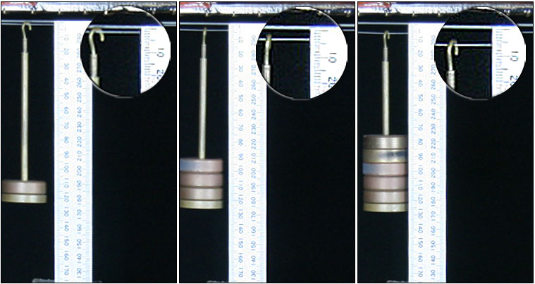
For small deformations, a
tightly stretched string is a linear medium: a displacement from its equilibrium position produces a restoring force that is proportional to the displacement. You can see from these photographs that, by this definition, a guitar string is approximately a linear medium, for deformations of a few mm. (The masses are 200, 400 and 600 g so the tensions are 2, 4 and 6 newtons.)
Linear superposition
We shall see later that, in linear media, the wave equations are relatively easy to solve. We shall see also that linear media exhibit linear superposition:
In a linear medium, if y1(x,t) and y2(x,t) are solutions to the wave equation, then
y1(x,t) + y2(x,t) is also a solution.
The rope used above was not a very linear medium: in order to slow the wave speed, we used a low tension, which meant that the tension depended on gravity and the angle of the rope. Also, the tension was low enough that the bending stiffness of the rope may have been important. So, to illustrate superposition, we use a torsional wave apparatus, which is more nearly linear than the rope.
This device has a stretched metal band (actually a used blade from a band saw), to which are riveted a series of bars, with yellow discs at each end. We show elsewhere that the wave speed in a stretched string is v = √(T/μ) = √(TL/m), where T is the tension, m is the mass, L the length and μ = m/L is the mass per unit length of the string. The speed of a torsional wave is v = √(K/i) = √(KL/I), where K is the torsional stiffness, I is the moment of inertia, L the length and i = I/L is the moment of inertia per unit length.
(See rotational mechanics.) The bars not only make small displacements easier to see, they also increase the moment of inertia and thus give a slow wave speed.
Notice the way the two waves seem to 'pass through' each other (use the step button). When the two pulses occupy the same region of x, we see linear superpostion: y = y1 + y2. We also see this when one of
y1 or y2 is zero, of course. The pulses are approximately the shape of a bell curve. So, in the animation below the clip, we show explicitly two travelling bell curves and their sum. The equations are
y1(x,t) = A.exp−(x−vt−x01)2 and y2(x,t) = A.exp−(x+vt−x02)2
where A is the amplitude, v the wave speed and x01 and x02 are the initial positions of the peaks of the two wave pulses.
The limits of linearity
In physclips, we shall consider only linear media explicitly. Further, many media are linear for waves of small amplitude. But what does 'small' mean in this context? With what should we compare the wave amplitude? In the case of the stretched string, there are two requirements: the amplitude should be small enough so that the slope θ due to displacement of the string allows the small angle approximation, sin θ ≅ θ and also that the increase in tension produced by the deformation is much smaller than that in the string at rest.
For a long wavelength wave in the ocean, there is an obvious vertical dimension with which to compare the displacement: the depth of the water. Some very interesting nonlinear effects happen near the beach, when the wave height becomes comparable with the depth of the water.
For a sound wave, there is an obvious pressure with which to compare the variation in pressure due to the sound wave: the pressure in the atmosphere in which the wave travels. Except for sounds that would deafen you, the pressure amplitudes in a sound wave are much less than atmospheric, so it is usually appropriate to treat the atmosphere as a very nearly linear medium for sound. If you are now wondering whether there is a linear limit for electromagnetic waves, the answer is yes. In media, of course, the field must be small enough so that it doesn't ionise or cause other chemical changes in the molecules of the medium. In vacuum, there is also a limit: the energy density of the wave needs to be low enough that it does not create particle-antiparticle pairs.
Reflections at fixed and free boundaries
The wave machine is shown in two configurations. In the top clip, the right hand end of the medium is fixed: a pair of clamps set the (angular) displacement to zero. In the bottom clip, the band is on a bearing: it and the bars are free to rotate at the right hand end. (This is another advantage that the wave machine has: it is difficult to arrange for string to be subject to a tension and still free to move at one end.) Observe what happens when the pulse arrives at the fixed end and at the free end.
Let's have a look at the reflection at a fixed end, this time comparing it with an animation. The animation shows, in black, the resultant motion of the string: compare it with the film clip, perhaps using the stop button. It also shows, in red, the incident wave travelling to the right and passing right through the boundary. It shows too, in blue, a wave with negative displacement that starts from the right, beyond the boundary, and travels to the left. This wave is a reflection of the incident wave in both the vertical and horizontal directions. So, at the boundary, the incident plus reflected add up to zero, which is the required condition at the boundary.
We can write that mathematically. Let's take the origin at the boundary. Let the incident wave yi and the reflected wave yr be given by
yi(x,t) = A.exp−(x−vt)2 and yr(x,t) = −A.exp−(x+vt)2
.
At x = 0 (at the boundary), the total wave y = yi + yr = 0, as required by the fixed boundary. For a free boundary, we would use yr(x,t) = +A.exp−(x+vt)2, so that we had maximal amplitude at the boundary. So we conclude that:
At a fixed boundary, the reflected wave is inverted.
At a free boundary, the reflected wave is not inverted.
Of course, boundaries are never entirely free, nor entirely fixed. So let's now look at reflection and transmission when there are finite discontinuities at the boundary.
Reflection and transmission at step changes in density
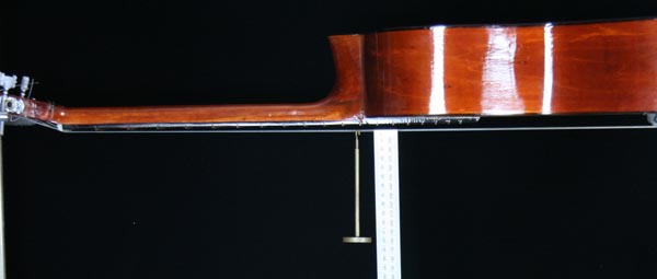
The still photographs below show the junction between a rope and a string. For each of these, we can define a line density, μ, with is the mass per unit length. The rope has μ = 27 g/m and for the string μ = 6 g/m. Because they are connected together, their tensions are the same. Let's see what happens when a wave passes from low density to high (left), and then low density to high (right).
Note that there will be reflections at three different places: at the junction between the two strings, at the distant post where the string is tied, and at the support point in the foreground. The foreground and distant points are essentially fixed boundaries.
First reflection. The
pulse starts on the right, travels to the light-to-heavy boundary, is inverted on reflection, and travels back on the left.
Foreground reflection. The reflected pulse, arriving on the left, meets a fixed boundary and is inverted on second reflection, so it now goes away from us on the right.
Transmission. Meanwhile, the initial incident pulse, on the right, has arrived at the light-to-heavy boundary. At the boundary, the two strings move to the right on its arrival, although not very much because the second string has such high μ. Nevertheless, this creates a transmitted pulse to the right: the transmitted wave is not inverted.
As the clip ends, both the transmitted pulse and the twice reflected pulse are travelling away from us, both on the right.
Although the tensions T are the same in the two strings, the line denstities μ are different, so the wave travels more slowly in the high string. We shall show later that v = √(T/μ).
First reflection. The
pulse starts on the right, travels to the heavy-to-light boundary, is not inverted on reflection, and travels back on the right. (Note the reduction in the size of the pulse: some energy has gone into the transmitted wave.
Transmission. The incident pulse, on the right, arriving at the heavy-to-light boundary moves the two strings to the right on its arrival, rather vigorously because the second string has a low μ. This creates a transmitted pulse to the right: the transmitted wave is not inverted. Travelling in the low μ medium, the transmitted wave travels rapidly.
Distant reflection. At the distant, fixed boundary, the transmitted wave, arriving on the right, is inverted on reflection. So it returns on the left.
Foreground reflection. When the first reflection wave gets to the foreground fixed boundary, it is inverted on reflection. This turns it into a pulse on the left. As the clip ends, this pulse from the foreground fixed boundary meets the the reflection from the distant fixed boundary.
Let's leave pulses for the moment, and let's look at another, very important waveform: the travelling sine wave
This web page supports the multimedia tutorials Waves I and Waves II. Most of the animations above may be downloaded from those sites.

 , a function of (x − vt). Now there is nothing special about this function, or the point we chose, so any function y = f(x−vt) is a wave travelling to the right with speed v and with unchanging shape f(x').