The speed of sound in air is approx. 340 m s-1, so we can generate velocities that are sufficiently large to produce modest but quite measurable Doppler shifts.
In these experiments we use a computer with internal microphone to record the sound from a moving source. (Having the microphone separate from the computer would have advantages over using the internal microphone, because we want high speed sources to pass close to the microphone, without endangering the computer. In this experiment, however, we were simply careful.) Comparison of the frequency measured for the source while moving with that measured with the source at rest allows the velocity of the source to be estimated.
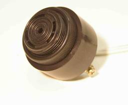
The sound source we will use is a standard piezo-electric buzzer or alarm – see figure 1.
Fig. 1. A standard piezo-electric buzzer
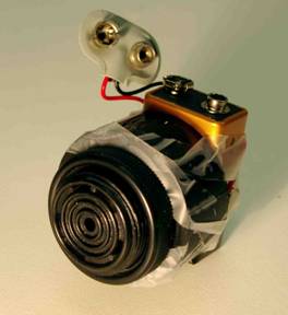
These are buzzers are physically robust and provide a stable, loud sound source at a single known frequency (usually around 3 kHz). They are widely used in items like reversing alarms on cars or smoke alarms. They are cheap and readily available from electronic shops for approx. $3 to $15. Our buzzer was powered by a 9V battery attached to its back with adhesive tape – see figure 2.
Fig. 2. Buzzer with battery attached
The software we used for sound recordings and the calculation of frequencies was Audacity. Audacity is free, open source software for recording and editing sounds and is available for several platforms including Windows and Mac OS X – see http://audacity.sourceforge.net/ . We used version 1.33.11 – it is a Beta version but appears to be completely stable (at least on my Mac). Audacity has useful help files and a manual on the web
The frequency of the source will be measured by examining its frequency spectrum. In general these experiments are best performed in the open air to minimise the complications caused by the standing waves that can be generated by reflections in a room.
Circular Motion
An easy way to produce high velocities is
to swing the sound source in a circle at the end of a rope.
Safety:
Even small objects can be highly dangerous if released at speed (remember David
and Goliath in the Bible). It must be impossible for the sound source to become
detached from the string while undergoing circular motion. I used a source
embedded in a polystyrene sphere borrowed from our Demonstration unit. However
placing the sound source in a string bag should be fine.
Measurements:
(1) Place notebook or laptop computer on the ground.
I chose a position close a nearby hedge. This had two advantages; (i) I could
arrange for the swinging source to hit the hedge before it hit my computer and
(ii) it made it harder for people to unexpectedly walk in the path of the
swinging sound source.
(2) Start your sound source and start the computer
recording sound.
(3) Let the computer record for a few seconds with
the source stationary; this allows you to measure the source frequency at rest.
(4) Now swing your sound source in a circular path
for several seconds. You should let it pass close to the inbuilt microphone in
the computer – see video.
(5) Take great care NOT to hit the computer
(6) Stop the computer recording the sound and
disconnect your sound source.
Analysis:
Your window in Audacity should display the
measured waveform and could look something like this figure taken from our
measurements. (This is a graph of sound pressure p as a function of time).
Play the sound of your waveform; you should hear a small periodic rise and fall in pitch as the sound source passes close to the microphone in your computer.
Here’s the sound we recorded.
(The whistling sound about half way through
the recording was caused by a ‘howling football’ thrown by nearby students).
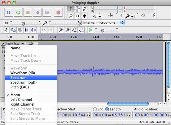
Now to measure how the frequency varied
with time.
Go to the ‘Audio Track’ pull-down window.
And select ‘Spectrum’ as shown below.
Audacity will now display a spectrogram -
a graph of the power at each frequency as a function of time. The vertical axis
displays frequency and the horizontal axis displays time. The power at each
frequency is indicated by the colour; power ranging from high to low is
indicated by white -> red -> blue.
Any such spectrogram is necessarily a
compromise between resolution in frequency and in time. If each point on the
spectrogram is calculated using a large number of data points the spectrogram
can indicate small changes in frequency, but the resolution in time will be
reduced.
For a given sampling rate (fsamp) and
number of data points (npts) the resolutions df in frequency and dt in time are
related by
df = fsamp/npts
dt = npts/fsamp = 1/df
The settings used to display the
spectrogram can be changed by pulling down ‘Audacity’ in the menu bar and
selecting ‘Preferences…’.
Here are the values I used for the
spectrogram shown below
And here is the spectrogram.
The variation in frequency measured by the observer is seen to vary periodically as the source describes its circular path. Note the asymmetric shape. The minimum frequency occurs soon after the source has passed the microphone (when a line from the microphone to the source is a tangent to the circular path). Thereafter, its receding velocity component decreases, to be zero on the opposite side of the circle. Then it starts approaching, with increasing velocity. So, from the receding tangent point to the approaching one, the frequency gradually increases. Then it abruptly decreases. (The decrease would approach instantaneous if the source passed very close to the microphone.)
(The frequency as measured by the experimenter swinging the source will not vary significantly with frequency because there will zero relative velocity between experimenter and source.) For the experiment shown above, the frequency varied between 3450 Hz and 3150 Hz, a difference of 300 Hz. The frequency measured at rest was 3290 Hz.
So Vs = (f’-f)v/f’ = (3450 – 3290) 340 / 3450 = 15.7 m s-1.
Similarly for receding = Vs = (f’- f)v/f’ = (3290 – 3150) 340 / 3150 = 15.1 m s-1.
Let see what we mighty expect from the kinetics of circular motion. The sound source was making 1.35 revolutions per second along a path of radius r = 1.7 m, so v would be given by v = rw = 2p if r = 14 m s-1.
The agreement is reasonable considering that there are several possible sources of error in this experiment.
Extensions:
The sound source could be swung on different lengths of rope to produce different angular velocities.
The shape of the periodic variation of frequency with time should vary with the distance between the microphone and the point of closest approach of the sound source.
Experiments under more controlled conditions are possible. Thus the sound source can be attached to a spinning wheel and arranged to pass very close to the microphone.
Linear Motion:Bicycle
Moving Source
In this experiment a sound source is attached to a bicycle which is ridden past a microphone.
Here is the measured spectrogram when Joe rode past the microphone.
The rapid decrease in frequency as Joe
passes and the microphone is immediately apparent. In this experiment the
frequency varied between approximately between 3025 Hz and 2880 Hz, a
difference of 145 Hz.
The spectrograms in Audacity have an upper
limit of 4096 samples. At the standard sampling rate of 44100 Hz (the sample
rate for an Audio CD) these samples will take a period of 4096/44100 seconds,
about 93 ms. The frequency resolution is thus 1/0.093 = 10.8 Hz. If we require
greater resolution in frequency, it is possible to achieve this in Audacity by
plotting the spectrum rather than a spectrogram. The upper limit for a spectrum
is 16384 samples that will take about 0.38 s and give a frequency resolution of
about 2.7 Hz.
To do this first select a section of your
waveform. The go to ‘Analyse’ in the menu bar and select ‘Plot Spectrum’ – see
figure
This is the result. It is a plot of power on the vertical axis as a function of frequency on the horizontal axis. It differs from a spectrogram in that there is now no dependence upon time.
Alas Audacity does not allow us to expand the frequency axis so we can easily determine the frequency that has the greatest power. However it does provide a cursor that shows the power at the frequency corresponding to the horizontal position of the cursor.
So now move the cursor very slowly around the 3 kHz region until the frequency with the greatest power is found (for this case it will be the smallest negative number). The movement can be very sensitive and sometimes I find it helpful to greatly extend the width of this window.
The number given by ‘Cursor:’ just below the frequency axis refers to the power at the particular frequency specified by the cursor.
The number given by ‘Peak:’ just below the frequency axis is the result of interpolation between the frequencies in the spectrum. You should use this value.
The peak values returned can depend subtly upon the particular section of the waveform that is examined. It is thus a good idea to plot spectra for several slightly different selections from the waveform to check they return the same result.
For the experiment with the moving source, i.e. attached to the bicycle, we measured the following values.
The frequency at rest was 2928 Hz.
So Vs = (f’-f)v/f’ = (2993– 2928) 340 / 2993 = 7.4 m s-11 = 27 km hr-1
Similarly for receding = Vs = (f’- f)v/f’ = (2928 – 2877) 340 / 2877 = 6.0 m s-1 = 22 km hr-1
So it appears that Joe very prudently started to brake once he passed the microphone.
Moving Observer
In this experiment the source was fixed
whilst the observer was a microphone in a video recorder.
You could alternatively use a smart phone or camera to record the
sound.
Here is the spectrogram
As expected it is very similar to that measured for a moving source.
Repeating the procedure for the moving source we found
For approaching Vs = (2996– 2932) 340 / 2996 = 7.3 m s-1 = 26 km hr-1
For receding Vs = (2932– 2875) 340 / 2875 = 7.3 m s-1 = 26 km hr-1
It appears that Joe was more confident of his braking distance for this later experiment.
We can check this speed because one of Joe’s brake pads rubbed against the fork every revolution of the wheel and the sound it made can be detected on the recording for the moving observer.
From the time it took for 9 revolutions of the wheel, the time taken for a single revolution was T = 0.294 s. The diameter of the wheel was 0.695 m, so Joe was travelling at v = pi*0.695/0.294 = 7.42 m s-1 = 26.7 km hr-1
The velocity measured via the Doppler shift is thus in reasonable agreement.
If you perform this experiment it might be a good idea to measure similarly the speed by attaching a piece of cardboard or stiff paper to the wheel so it makes a noise every revolution. Indeed if you attach a piece of card to the fork so it hits the spokes you might even be able to use the sound it makes instead of a buzzer.
LINEAR MOTION. Running:
In this experiment John held the sound
source and ran towards the computer.
Here is a spectrogram of the recorded
sound.
A gradual increase in frequency over the first few seconds as John accelerates is apparent followed by a sharp decrease just before 5 seconds as John passed the microphone. However we can find the frequency a little more accurately using the spectrum.
The frequency at rest was 2806 Hz and reached a maximum value of 2850 Hz.
So Vs = (f’-f)v/f’ = (2850– 2806) 340 / 2850 = 5.2 m s-1 = 19 km hr-1
LINEAR MOTION. Walking
In this experiment John held the sound source and walked as fast as he could towards the computer.
The frequency at rest was 2806 Hz and reached a maximum value of 2833 Hz.
So Vs = (f’-f)v/f’ = (2833– 2806) 340 / 2833 = 3.2 m s-1 = 12 km hr-1
However as the speed is reduced, the frequency shift is correspondingly smaller and it approaches the limit of what can be reliably measured using Audacity. However if software is available that uses a larger number of samples, very small shifts in frequency can be detected.