How do pressure, density and particle speed vary in a sound wave? This is a support page to the multimedia chapter Sound. It gives background information to illustrate the differences between transverse and longitudinal waves, how these are notated and how longitudinal displacement in a sound wave leads to variations in density and pressure. This page is only illustrative: the analysis continues on The wave equation for sound.
In a transverse wave, the particle displacement is at right angles to the direction of wave propagation. Here, the wave in the spring travels to the right, while the displacement is largely vertical, so this is a largely transverse wave.
The wave shown below is largely longitudinal. The coils of the spring are displaced left and right; parallel then antiparallel to the direction of propagation. At any time, the displacement of coils have different values. This produces variations in density. We see that a region of high density travels along the spring, first to the right then to the left.
y(x') in a longitudinal wave
In the transverse wave, we used y(x) for the (transverse) displacement as a function. In that wave, as usual, y was at right angles to x. In a longitudinal wave, we still use y(x) for the displacement, and this animation shows how that works. As we did in Travelling Waves I, we use x for the coordinate in the stationary frame, and x' for the coordinate in a frame moving with the wave, at v to our x frame.
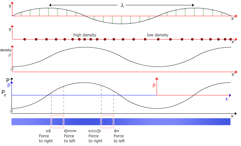
The top graph plots y(x'). On the axis below, we add these displacements y, and we rotate the arrows clockwise so that positive displacement is to the right and negative to the left. We then apply these displacement to the particles, which were initially equally spaced. Once the particles are displaced longitudinally, we see that there are regions of high and low density. Density is plotted on the next axis. Notice that, for a sine wave, the maxima and minima of density correspond to zeros in y(x').
For a wave in a gas, high and low density correspond respectively to high and low pressures. The absolute pressure P varies little in a sound wave: the small variations from atmospheric pressure is called the acoustic pressure, p. At the bottom of the panel, we represent the density variation by (exaggerated) variations in colour density.
A travelling wave
In all the plots above, we have showed y(x'), where x' is the coordinate moving with the wave. If the x' frame is travelling to the right at speed v, then the coordinate x in the fixed frame is x = x' + vt, In this animation, we show the wave in the x frame.
Pressure differences and nett forces
Why should a wave propagate? If the pressure varies as a function of position, then some regions of the medium will be subject to a nett force. The two sections highlighted by the pink boxes show regions of the medium subject to nett forces.
The next step is to analyse the wave. To relate pressure to density, we need to know a little about the elasticity of the medium, which is often a gas. To relate the motion of the medium to the spatial variations in pressure, we need Newton’s second law. That’s what we do next, on The wave equation for sound.