This is a support page to the multimedia chapter Oscillations. It gives background information and further details.
Oscillations are important in their own right. They are also involved in waves. This movie clip shows a torsional wave – first a travelling wave, then a standing wave. The oscillation of one point on the wave is highlighted.
We discuss it below. (This page has many film clips and may be slow to load.)
In the slow motion movie clip at right, the mass glides on an air track. The track is perforated with small holes, through which flows air from the inside, where the pressure is above atmospheric. So the mass is supported, like a hovercraft, on a cushion of air, and friction is eliminated. Because the speed is small, air resistance is very small. Consequently, the only non-negigible force in the horizontal direction is that exerted by the two springs. Because there are no vertical displacements, we discuss here only the horizontal displacement.
At the equilibrium position (x = 0 in the graph below the clip), the forces exerted by the two springs are equal in magnitude but opposite in direction, so the total force is zero.
To the right of equilibrium, the force acts to accelerate the mass to the left, and vice versa.
(The graph is rotated 90° from its normal orientation so that we can compare it with the motion.)
Let's begin (as do the graph and the animation) with the mass to the right of equilibrium and at rest. Let's see what happens when I release it:
First, the spring force acts to the left and mass is accelerated towards x = 0.
When it reaches x = 0, it has a velocity and therefore a momentum to the left. (Near equilbrium, the forces are small, so there is a region near x = 0 over which the velocity changes little: the x(t) graph is almost straight.)
When it arrives at x = 0, because of its momentum to the left, it overshoots, i.e. it continues travelling to
the left. While it is to the left of x = 0, however, the spring force acts to the right. This force gradually slows the mass until it stops. The point at which it stops is, of course, its maximum displacement to the left.
Once it is stopped on the left hand side of equilibrium, the spring force accelerates it to the right, so the velocity and momentum to the right increase.
When it reaches equilibrium again, it now has its maximum rightwards momentum.
It overshoots and continues to the right. The spring force now acts to the left, so it decelerates until it stops at its maximum rightwards displacement.
For linear springs, this leads to Simple Harmonic Motion. The force F exerted by the two springs is F = − kx, where k is the combined spring constant for the two springs (see Young's modulus, Hooke's law and material properties). In this case, k = k1 + k2, where k1 and k2 are the constants of the two springs. The analysis that follows here is fairly brief. However, we do a quantitative analysis on the multimedia chapter Oscillations and also solve this problem as an example on Differential Equations.
There is also a page on the Kinematics of Simple Harmonic Motion.
Newton's second law states that the acceleration d2x/dt2 of the mass m subject to total force F satisfies F = m.d2x/dt2 , which gives the differential equation
m.d2x/dt2 = − kx, or d2x/dt2 = − ω2 x , where ω2 = k/m .
Solving this particular equation is described in detail on the Differential Equations page. However, we can verify by subsitution that the solution is
x = A sin (ωt + φ),
where A is the amplitude, and the phase constant φ is determined by the initial conditions. We discuss these below.
In the first movie shown shown at right, the mass is released from rest,
so the amplitude is maximal (x = A) at t = 0, so the required phase constant is φ = π/2. (Indeed, for this particular case, we could say that the curve is a cos function rather than a sine.)
x1 = A sin (ωt + π/2) = A cos (ωt )
In the second movie shown at right, however, the mass is given an impulsive start, so the initial condition approximates maximum velocity and x = 0 at t = 0. This requires φ = 0, so
x2 = A sin (ωt + 0) = A sin (ωt)
Here we start with an initial velocity, which is
v0 = dx2/dt = A sin ωt = Aω
Note that the initial condition determines both φ and A.
In both these clips, a rotating line (an animated phasor diagram) is used to show that Simple Harmonic Motion is the projection onto one dimension of circular motion. This is explained in detail in the Kinematics of Simple Harmonic Motion in Physclips.
Phasors are commonly used to facilitate calculations in AC circuits.
We saw above that x = A sin (ωt + φ), where ω2 = k/m .
The cyclic frequency is f = 1/T, where T is the period. The sine function goes through one complete cycle when its argument increases by 2π, so we require that (ω(t+T) + φ) − (ωt + φ) = 2π, so ωT = 2π, so
ω = 2π/T = 2πf = (k/m)½ .
This parameter is determined by the system: the particular mass and spring used. For a linear system, the frequency is independent of amplitude (see below, however, a for nonlinear system ).
Compare the oscillations shown in the two clips at right. The first uses one air track glider and the second uses two similar gliders, so the mass is doubled. The period is increased by about 40%, i.e. by a factor of √2, so the frequency is decreased by the same factor.
Though it is not so easy to see in the video, at right we have used stiffer springs with a higher value of k. Here the period is shorter and therefore the frequency higher that in all the previous examples.
Because we know x, the displacement from equilibrium, we know the potential energy U, which is just that of a linear spring. Taking the zero of potential energy at x = 0, U = ½ kx2. Here,
x = A sin (ωt + φ) so
U = ½ kx2 = ½ k A2 sin2 (ωt + φ).
Because we know v, the velocity in the x direction, we know the kinetic energy K.
v = ωA cos (ωt + φ) so
K = ½ mv2 = ½ m ω2A2 cos2 (ωt + φ).
Adding kinetic and potential energies gives the mechanical energy, E.
Using the expressions above, and substituting ω2 = k/m
, we have
E = U + K = ½ kx2 + ½ mv2 = ½ kA2 cos2 (ωt + φ) + ½ k A2 sin2 (ωt + φ).
Now we can use the identity sin2 θ + cos2 θ = 1, which gives
E = U + K = ½ kA2,
which is a constant: it does not depend on time. This is because of the air track: here, no non-negligible nonconservative forces act, so mechanical energy is conserved.
U (in purple, like x), K (in red, like v) and E (in black) are shown as functions of time in the animated graph at right: the mechanical energy is continuously exchanged between potential and kinetic.
At the extrema of the motion, where |x| = A, the velocity is zero, so
This is a movie clip of the Foucault Pendulum in the School of Physics at UNSW. (The purpose of that pendulum is to demonstrate that the earth is not an inertial frame, but has a centripetal acceleration due to the rotation of the earth on its axis. Because the earth rotates clockwise (viewed from the South), the plane of the pendulum's swing precesses very slowly anticlockwise.)
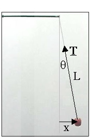
A mass m hangs from a light, inextensible string of length L, which is large+ compared to the dimensions of the mass, so the mass can be considered as a particle. The horizontal displacement of m from the position of equilibrium is x, and the string makes an angle θ with the vertical, as shown in the sketch. For the moment, we consider only the case in which θ is small, so x << L.
Applying Newton's second law in the vertical upwards direction, we have*
|T| cos θ − mg = may
Because θ is small, the vertical acceleration ay is negligible. Further, cos θ, which may be expanded as cos θ ≅ 1 − ½ θ2 +..., is approximately 1. So the magnitude |T| of the tension in the string is approximately mg.
Applying Newton's second law in the horizontal direction,
− |T| sin θ = max = m d2x/dt2.
Then we write sin θ = x/L.Substituting this in the preceding equation and rearranging gives
d2x/dt2 = − (g/L)x or
d2x/dt2 = − ω2 x, where we define ω2 = g/L.
This, of course, is the differential equation we have solved above and elsewhere. Its solution is
x = A sin (ωt + φ), where ω = (g/L)½
Writing T as the period (not to be confused with the magnitude of the tension |T|), we write 1/T = f = ω/2π = (1/2π)(g/L)½.
Here, the potential energy is gravitational. If we take the lowest point of the pendulum (y = 0) as the reference of U, then, making the same substitutions as above,
U = mgy = mgL(1 − cos θ) ≅ mgL(1 − (1 − ½ θ2)) so
U ≅ ½ mgx2.
The energy terms are illustrated with histograms at right. The reference for potential energy is arbitrary, as we have suggested in the animation.
+The importance of this condition is that its rotational kinetic energy can be neglected in comparison with its translational kinetic energy and gravitational potential energy. We shall also neglect the slow rotation of the earth.
* Notice that, in this equation, we have used the symbol 'm' in two conceptually different ways: the m in mg is the gravitational mass, the quantity that interacts with gravitational fields. The m in ma is the inertial mass, the quantity that resists acceleration. See this link for more discussion.
Pendulums are easy to make and their periods can be measured accurately. Further, because they are only simple harmonic oscillators in the small angle approximation analysed above, they provide a good system for showing the effects of nonlinearity. That is the purpose of the movie clips below, which show how, for the nonlinear oscillator, the period varies with amplitude and, at large amplitudes, the motion is not sinusoidal.
This is an example of an oscillation that is harmonic, but not simple harmonic. Periodic motion is motion that repeats: after a certain time T, called the period, the motion repeats, or x(t+T) = x(t). Periodic motion is called harmonic motion and may be expressed as a sum of harmonics. We shall discuss harmonics later, when we meet standing waves in one dimension. Mean while, see What is a sound spectrum? and How harmonic are harmonics?
In practice, nonconservative forces are usually present, so mechanical energy is lost over each cycle. The type of loss that is most commonly analysed is that produced by a force proportional to the velocity, but in the opposite direction.
Analysing that case in one dimension, we would write
Floss = − bv = − b dx/dt.
Let's add this term to the analysis given above. Newton's second law is Σ F = m.d2x/dt2 , which gives the differential equation
m.d2x/dt2 = − kx − b dx/dt, or
d2x/dt2 + 2β dx/dt + ω02 x = 0 , where ω02 = k/m and β = b/2m.
We can verify by subsitution that this differential equation has a solution
x = A e−βt sin (ωt + φ), where ω2 = ω02 − β2.
So, for this particular damping force, we should expect an oscillation whose amplitude decreases exponentially with time.
Forces proportional to velocity arise from the viscosity of simple Newtonian fluids, if motion is sufficiently slow. However, losses encountered in nature are frequently more complicated. In the case below, the pendulum is mounted on a roller bearing. The loss force in this case has a dependence on v that is less strong than proportionality.
What is happening here? Why is the decay faster than exponential? Liquids with long chain molecules frequently exhibit non-Newtonian viscosity. When the velocity gradient is large enough, shear forces tend to align the molecules at right angles to the velocity gradient, which reduces the viscosity. I speculate that the grease in the bearing
is behaving in this manner. The relative infrequency of linear losses in condensed phases is mathematically inconvenient, because the linear equation is much easier to handle analytically.
Linear damping does exist, but real systems are rarely that simple.
In the analysis above, we have included the restoring force (spring in the first case, gravity for the pendulum). Other, time-dependent forces may also be present. We could include these as F(t) and write
Analysing that case in one dimension, we would write
d2x/dt2 + 2β dx/dt + ω02 x = F(t)/m .
The externally applied force F(t) might be a simple oscillation or might have oscillating components. This gives rise to the phenomenon of resonance.
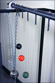
The apparatus shown at right has a set of pendulums of different lengths attached to the same shaft via rods that rotate with the shaft. On the far end of the shaft is a pendulum with much larger mass, similarly attached. The oscillation of the massive pendulum tends to rotate the shaft at an angular frequency ω = (g/L)½, where L is its length.
This rotation produces an external, time dependent force on each of the small pendulums, each of which has its own characteristic frequency ω0. While the movie clip is downloading, make a prediction of what you think will happen to the small pendulums.
How will the work done be this external force depend on ω0? If the force is applied in the same direction as the motion, then the work done will be positive. If ω ≠ ω0, then we might expect that, over several periods, there would be some periods for which the velocity and the external force were in the smae direction, but these would tend to cancel out. On the other hand, if ω ≅ ω0, and if the phase between them were suitable, we can imagine cases where the work done over several cycles would be large. ω0 is called the resonance frequency of the system.
The two clips below show the importance of the frequency and phase of the external force.
Let's be quantitative, by adding an external force
(F0 sin ωt) to our previous analysis, which yields the equation
d2x/dt2 + 2β dx/dt + ω02 x = (1/m) F0 sin ωt .
where again ω0 = k/m. As written, this equation applies to an external force applied over a very long time: we have made no mention of when and how the force starts. So let's consider what happens in the quiescent state, the state over which the average work being done by (F0 sin ωt) equals the average rate at which energy is being dissipated by the nonconservative force (Floss = − bv = − (2β/m) dx/dt). We can verify by substitution that the solution to this equation is
x = A sin (ωt + φ), where A =
(F0 /m)((ω2 − ω02)2 + (2βω)2)−½
and where tan φ = 2βω/(ω2−ω02).
Note that, in this quiescent state, the amplitude is large if ω0 ≅ ω0 and if the loss term, β/ω0 is small, i.e. if dissipative forces are not doing work at a large rate. At resonance (i.e. when ω = ω0), the amplitude is A = F0/2βωm.
Sometimes the loss term, βω, is hard to measure directly, so instead we measure the Quality factor, Q, defined as Q = ω0/Δω, the ratio of the resonant frequency to the bandwidth, where Δω is the difference between the frequencies that give half maximum power, or amplitudes reduced by √2. Using the expression above for A, the half power points occur when ω½2 − ω02 = 2βω. Solving this quadratic gives ω½ = β ±√(β2+ω02). For reasonably high Q, i.e. when Δω << ω0, this allows the approximation ω½ ≅ ω0(1±β/ω0), which gives β ≅ 2ω0/Q. This then gives the amplitude at resonance as A0 ≅ F0Q/(4mω02) = F0/(4mω0Δω). This makes qualitative sense: the amplitude is obviously large for large F and small m, it is small at high frequency when there is not enough time per cycle to displace it much, and large if the resonance is strong, i.e. if the Q factor is high or the bandwidth low. The phase between the driving force and the steady response is φ = tan−1(ωω0/Q(ω2−ω02)). So at resonance, the force leads the displacement by π/2 and is in phase with the velocity.
These expressions apply to a system with linear losses, where the dissipative force is proportional to velocity, as is the case for vicosity. The nonlinear losses that one often meets in practice yield equations that (e.g. dynamic drag) are rather more difficult to solve and are not treated here. In the equation above, φ is the phase by which x(t) is ahead of F(t). At low frequency (ω << ω0), φ is near zero: negligible force is required to accelerate the mass, so the driving force simply pushes the spring: applied force F = kx. Conversely, at high frequency (ω >> ω0), φ is near 180° and the force and displacement are in antiphase: the driving force is in phase with the acceleration, because the acceleration term dominates when ω is high. At resonance (ω = ω0), φ = 90° and the driving force is in phase with the velocity.
We do not discuss here the transient behaviour: the way a system responds when the external force is 'turned on' or 'turned off'. Examples are shown, however, in the movie clips above.
We have treated the mass on springs and the pendulm mass as though they were particles: objects with no size or zero dimensions. The displacement of a particle can be written as x(t), a function of time alone. For extended objects that are not completely rigid, there is the possibility of oscillation with amplitudes and phases that vary within the object. A simple example is an ideal string, extended in the x direction, whose transverse displacement can be written as y(x,t).
This animation shows a wave travelling to the right (green line) and another, of equal frequency and amplitude, travelling to the left (blue line). In a linear medium, these add to give a standing wave, shown here as a red line that represents (with the vertical scale exaggerated) a wave on a string fixed at the position of the two vertical lines. The physics and musical applications of strings are discussed in Strings, standing waves and harmonics from our Music Acoustics site.
The movie clip below shows a wave in a one-dimensional medium.
The waves in this clip are torsional waves θ = θ(x,t). The straight line across the image is a strip of steel (a blade from a band saw), to which are attached the long arms that make the angular displacement visible. For convenience, the gravitational field has been rotated 90° in this clip.
We shall study these effects in the chapter on standing waves. For the moment, however, let's look quickly at other examples.
In three dimensions, we can exite oscillations with displacement ξ = ξ(x,y,z,t).
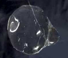
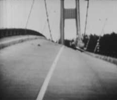
In general, this is hard to show on a two-dimensional screen, except in animation. The clip drop of water shown below at left was made by Don Pettit in free fall, in the International Space Station. The motion is complicated, but slow because the restoring force is the surface tension of water, which is rather small on this scale. The clip linked below right is a very famous film, regularly used to remind engineering students of the importance of resonances in structures.