Interference: Young's experiment with single photons
Young's two-slit experiment, one photon at a time: Shall we still see the classic interference pattern if the light level is so low that there is only one photon in the apparatus at a time? Which of the slits does the photon go through? If it goes through one, how does 'know' about the other? Or does it interfere with itself? Let's conduct the experiment and see. First, however, you may want to see the Introduction to Young's experiment in which we explain Young's experiment and calculate the intensity as a function of angle.
This page supports the multimedia tutorial Interference.
At left is a very dim lamp. A thin slit allows only a small fraction of its light into the apparatus, and this is filtered so that a further small fraction of photons is admitted. Then a single slit. This diverges the beam due to diffraction, and also further reduces the intensity (the number of photons per unit area per unit time). This weak beam of light reaches the plate with the double slit. Behind this is a moveable baffle, mounted on a micrometer. Turning the micrometer allows the baffle to cover one of the double slits, thus converting from a double to a single slit apparatus. Instead of a screen, the patter is formed on another baffle, whch has a small slit, behind which lies a photomultimplier tube (PMT). This baffle is mounted on a micrometer so the slit can be scanned across the interference pattern. Thus the PMT can measure the photon arrival rate at different positions on the interference pattern.The whole is in a light-tight box.
Close-up photographs
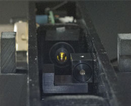
The photos below show some of the components of the aparatus.
Looking along the box towards the filter and the lamp.
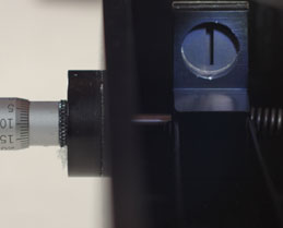
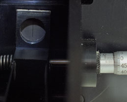
The moveable baffle with the micrometer drive that can cover one of the two slits.
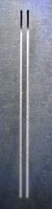
The two slits
The scanning slit and the micrometer drive that is used to scan across the interference pattern
Single slit diffraction pattern
With Flash animations no longer supported, run the tutorial movie from 1m20 to 1m30 (editing assistance sought). The background photo shows the light-tight box, with the lamp end at the left. In the midde is the micrometer that positions the baffle to expose one or two slits. At right is the box containing the photomultiplier tube. In the foreground is a movie showing the screen of an oscilloscope that displays the rate of photon capture as the scanning slit is moved across the pattern.
When a single photon strikes the electrode of the photomultiplier tube, it ejects a single electron. That electron is accelerated by a large potential difference so that, when it strikes another electrode, it has sufficient energy to eject many electrons. This process allows a single photon to produce an electric current pulse.
The PMT output is amplified and input to a loudspeaker. So each of the clicks that we hear in this movie records the arrival of a single photon. There are as many as several hundred photon arrivals per second, so only milliseconds between between them. However, the photons take only two nanoseconds to travel from lamp to PMT. Further their coherence length is small. So there is only ever one photon in the apparatus at a time.
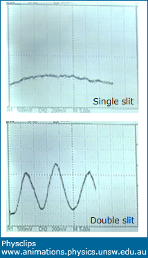
The PMT output is also amplifed, integrated and input to an oscilloscope, whose screen we see in the foreground movie above. The baffle covers one slit, so this movie shows the pattern produced by diffraction through a single slit.
Double slit interference pattern
For the movie shown below, the baffle has been moved to expose both slits. During the movie, the scanning slit is moved across the interference pattern.
The still at left shows the single slit diffraction pattern. The second screen movie shows the PMT output as the scanning slit is moved across the two slit interference pattern at approximately constant speed. With Flash animations no longer supported, run the tutorial movie from 1m30 to 2m10.
In this movie, we can both see and hear maxima and minima in the rate of arrival of photons at the PMT. The result shows the combination of diffraction and interference: a classic pattern for a two-slit Young's experiment. (For those who have noticed that the spacing between the peaks is not exactly equal: the answer is that the micrometer is moved by hand. The oscilloscope trace moves with constant speed and, if the micrometer speed were constant, this would mean that position on the oscilloscope screen is linear related to position on the interference pattern.I tried to keep the scanning speed constant by turning equal amounts in a regular rhythm, but the former is hard to achieve with precision.)
How to interpret this pattern? The oscilloscope trace in this experiment is a histogram of photon arrivals as a function of position across the 'screen'. So the interference term – the (cos 2φ/2) term determines the probability of photon arrival at any point. The square of the amplitude of the sum of the wave amplitudes determines the probability of photon arrival. Further, as we'll see later, a similar conclusion applies to electron behaviour.
From two slits to one slit at an interference minimum
Throughout the movie in the third screen, the scanning slit is positioned at a minimum in the interference pattern. During the movie, the baffle is moved so as to uncover the second slit: we go from two slits to one. With Flash animations no longer supported, run the tutorial movie from 2m10 to 2m35.
This time it is the baffle that we move with its micrometer. We go from two slits to one by covering one slit. With only one slit open, only half as many photons can get through the central screen. And yet, at this point, when we reduce the number of photons getting in, there are more photons detected. (Note: this is only true at points of destructive interference.)
From one slit to two at an interference minimum
Throughout the movie in the fourth screen, the scanning slit is positioned at a minimum in the interference pattern. During the movie, the baffle is moved so as to cover the second slit: we go from one slit to two. With Flash animations no longer supported, run the tutorial movie from 2m35 to 2m55.
Again, we move the baffle, this time covering one of the slits, thus going from one slit to two. This time, we double the number of photons passing through the central screen, but, at the position of our detector, there are fewer photons detected. (Again, this is only true at points of destructive interference.)
The photon questions
Light has properties associated with a wave (e.g. interference and diffraction) and properties associated with particles (local interactions, quantised properties). For many of us, 'photon' connotes particles. So, thinking about a particular photon that gave rise to one of the clicks we heard, we may ask: which slit did it go through? And, if it went through a slit, why is there interference? How did it 'know' about the other slit?
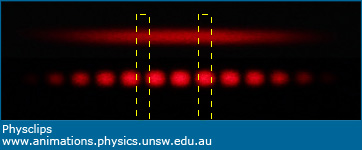
The difference between single and double slit patterns is readily explained using the wave model for light and we have done so in Introduction to Young's experiment (whence comes the next figure). At a point of destructive interference (e.g. yellow rectangle at left), the electric field components from the two slits are 180° out of phase, so they cancel out, which gives zero intensity. And zero intensity means zero photons. At a
point of constructive interference (yellow rectangle at right), the
electric field components from the two slits are in phase, so the fields add. Twice the field magnitude means four times the intensity, and for times the intensity means four times as many photons. So, with two slits, we have four times as many photons at maxima, no photons at minima and, integrated over the whole pattern, two slits has twice as many photons.
From a different experiment: the single slit diffraction pattern (top) and the two slit interference pattern (bottom).
It's worth saying that this cancellation in destructive interference is not something special about electric fields or quantum mechanical wavefunctions: it comes from the fact that, in waves, variables have phase as well as amplitude. We saw similar interference patterns when we conducted Young's experiment with water waves in Introduction to Young's experiment. So it works for water waves and light. And also for electrons:
Young's experiment with electrons
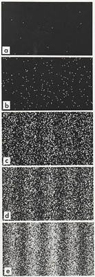
A group from the lab of Akira Tonomura performed an analogous experiment with electrons: Young's experiment, one electron at a time, from which we take the following images.
Successively longer integration times as electron arrivals (white dots) are recorded.
In the first image, it seems that the electron arrival is purely probabilitistic. The later images show that, as more and more electrons arrive, their 'histogram' gradually builds up the classic cos 2
interference pattern. Once again, the calculated intensity of the interfering waves (here, interfering matter waves)
gives the probabilty
of arrival of electrons coming from the two slits.
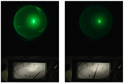
The next images are also made by interfering electrons, and they come from our next chapter on Diffraction. A beam of electrons passes through polycrystalline graphite and the interference pattern on the phosphorescent screen shows a pattern of interference – a little like the Bragg patterns that we'll meet in the next chapter. Further, we'd expect that the size of the pattern depends on the wavelength of the electrons.
Electron diffraction through a crystal
So what is the wavelength of an electron? And why and how does it depend on the acclerating voltage? We'll leave that until later chapters.
Is there a paradox?
What is sometimes called the wave-particle paradox/ puzzle/ mystery arises usually if we try to picture light or electrons or other tiny things in terms of macroscopic, familiar objects. If we imagine light as being like a water wave, it's impossible to picture how a photon is both dispersed enough to create an interference pattern and simultaneously localised enought to interact violently with a single electron. If we imagine light as being made of little particles, it's impossible to picture how one particle 'goes through' two slits and interferes with itself.
Light is not a water wave, and it's not a stream of little particles. Whenever we use one or other of these pictures (and they are very useful at times), we have to be aware that they are also, at times, seriously misleading. Further, the conditions under which one picture is helpful are usually those under which the other is misleading. Consequently, using both pictures simultaneously leads to apparent paradoxes. So it's good to remember that the paradox lies in the use of inappropriate, imagined, macroscopic pictures, and does not come out of the laws of physics.
I've been asked why this is so – why don't the laws of physics give a paradox. The answer has to do with the way science works. If two different scientific theories or ideas predict two different outcomes, then scientists would work very hard to perform that experiment. One or other (or even both) of the predictions would be found to be false, and that theory or idea would ultimately be either abandoned or else retained as a useful approximation for use only in some cases. So, for example, where Galilean and Einsteinien Relativity predict different answers, we recognise that Galilean Relativity is wrong in a fundamental sense. Nevertheless, we still use it as an approximation in most situations just because it makes calculations much easier. More about this in our volume on Relativity and more again when we come to quantum mechanics.