Lissajous figures

• The lab setup
• Some measurements and sound files

This Lissajous figure has 400 Hz on the horziontal (y₁ or x) axis and 500.1 Hz on the vertical (y₂ or y) axis. (This nomenclature is for consistency with the other web pages involving combinations of sine waves.) The slightly incommensurate ratio is chosen so that the phase changes gradually, as can be heard by the constructive and destructive interference in one of the sound files below.

By tracing the curve mentally, one can observe that, in four horizontal oscillations, there are five vertical oscillations. One can also determine this ratio by counting the number of intersections with the two axes.

More examples are given below.

The lab setup

The photo below shows a bench in the second year electronics teaching lab at UNSW, as we set it up for shooting some sequences for Beats, Tartini tones and Linear and nonlinear superposition, Consonance and phasor addition.

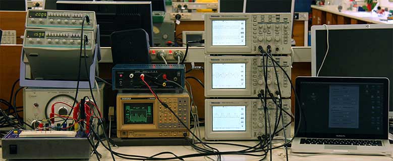
There are three oscillators at left, but we didn't use them: instead, we used the Physclips two-channel sine generator that you can download from the Oscillations Lab, which is running on the laptop at right. The latter is much more stable, precise and the two outputs may be phaselocked. At bottom left, below the oscillators, is a breadboard for making up simple circuits for linear and nonlinear superposition.

There's a stack of three oscilloscopes just to the right of centre. An oscilloscope usually displays voltage as a function of time and usually (as here) has two channels, so that you can plot V₁(t) and V₂(t). The scale of the vertical voltage axes can be set with knobs. The time axis is controlled with another knob: the 'timebase'. (In the old days of analogue Cathode Ray Oscilloscopes, this literally controlled the speed with which the electron trace passed from left to right of the the screen. We still hear people referring to oscilloscopes as CROs.)

The two channels from the oscillator drive the two channels on the top machine, and the one below shows the interaction of the two signals. In the case of Lissajous figures, this oscilloscope used one oscillation as the x input and the other as a the y input. (For other cases, this scope often showed their sum, but sometimes a non-linear combination) using the same time axis as the first scope. The third oscilloscope allows us to show the interaction of the two signals on a different way: usually with a slower timebase.

To the left of the oscilloscopes is a fourier analyser. (The large number of harmonics on its screen tells you that, for this photograph, we were using non-linear superposition.) Above that is an audio amplifier connected to a loudspeaker. This was connected to the combination signal but only for our convenience: the audio signal that you'll hear on Physclips was recorded directly from the electrical circuit and is only turned into sound in your sound system.

An oscilloscope needs to be 'triggered' to start a trace. In these experiments, we sometimes used the first channel (y₁) as a trigger. Otherwise, we used the 'line' trigger: a new trace was triggered in phase with the nominally 50 Hz power supply. This often varies slightly from 50.00 Hz, so it is not exactly synchronous with e.g. the 400 Hz signal from the computer.